Flight Customer Satisfaction

A Machine Learning Project to predict customer satisfaction for flight customers.

Introduction

Air travel has been, without a doubt, one of the biggest contributors to the world’s globalisation prospects in recent years. Not only did it revolutionise warfare, but it has also revolutionised transport and travel and given rise to multi-billion-dollar companies that employee millions of people. However, the recent and still ongoing Covid-19 pandemic has threatened this multi-billion-dollar industry due to the abrupt and sudden disruption to the way the world operates almost overnight. With these challenges, many airlines are now facing an uphill challenge to restore their previous levels of sales and compete in a depleted market against other airlines to carry the few passengers that are flying after the pandemic. When competing with multiple other companies providing the same services, the only way to make your mark is to have the backing and support of your customers. To ensure that this is the case, airlines need to ensure that customers are satisfied with the services being provided to them on their journey. For this reason, investment in data analytics has become a strong recommendation from various experts in the field. This study also aims to address this issue by using machine learning to identify which customers are more likely to be satisfied based on various indicators and experiences by the passengers themselves and which among them are more likely to be dissatisfied by the services. Modelling after a US airline passenger satisfaction survey conducted in 2015(John, 2016), this paper will implement three machine learning models of varying degrees of complexity starting with a Naïve Bayes Classifier, Decision Tree, and lastly an Artificial Neural Network. After the tuning and implementation of the model, the paper will evaluate the performance of these three models against each other based on their accuracy, sensitivity, specificity, f measure, Receiver operating characteristic (ROC) curve and Area Under the Curve (AUC).

Problem Statement

Covid-19 pandemic has disrupted the global travel industry to a previously unforeseen level and market competition between airlines has increased significantly in the depleted market. For this reason, the airline industry is in need of a solution cater to the business needs of the airlines to attract more customers to the airline. One way to stand apart from the competition is to ensure that passengers are satisfied with the services they receive on the airline to incentivise them to return to fly again or recommend the airline to others.

Aims and Objectives

The main aim of this paper is to develop a Machine Learning algorithm to predict customer satisfaction of airline passengers based on the flight features and customer feedback. To reach this aim the following objectives have been set.

• Conduct an Exploratory Data Analysis of the dataset o This will allow to identify missing and inconsistent data in the dataset and expedite and systemise the pre-processing of the dataset.
• Pre-Process and normalise the dataset to prepare it for Machine Learning o Pre-processing involves cleaning the data including filling missing values as well as normalisation and balancing of the dataset to ensure that the best results are obtained from the model.
• Implement three different Machine Learning models (Naïve Bayes, Decision Tree and Artificial Neural Network) o Implementing the algorithm includes training them on the same training dataset and tuning them based on their hyperparameters to obtain the best performing model.
• Evaluate the Machine Learning Models and identify the best performing model o Evaluation of the models include comparing the performance of the models based on different metrices such as accuracy, ROC and AUC.
• Identify the most significant factors that contributed to the prediction o Based on the performance of the best algorithm, the weights that contribute the most to the over all predictions will be identified to allow airlines to focus more on these features.
• Compare the ML models against previous models identified through Literature Review o This aspect of the paper will compare the best model created in this paper to other implementation found elsewhere on the same or similar datasets
• Recommendations for the future o The recommendations will include areas to improve on future implementations as well as recommendations for the businesses to improve customer satisfaction.

Scope

Due to the large dataset available for the problem at hand, the training time for the model will be unrealistically high for a study of this magnitude, especially when doing k-fold cross validation on each model including complex models such as Artificial Neural Networks and tuning each model. Hence, to ensure that the training time for models is realistic, a sample from the dataset will be taken to train and test the model.

Methodology

One of the most important steps to implement a Machine Learning algorithm for prediction is to outline the exact methods that will be used for the process. This section will explore the dataset that will be used for this purpose including it’s features and size followed by the description of the data pre-processing techniques and Machine Learning Algorithms that will be used including the specific libraries and why these algorithms were chosen. Lastly, we will explore the evaluation metrics that will be used to assess the performance of the three different models. The dataset to be used for this project is a US airline passenger satisfaction survey conducted in 2015 (John, 2016). This survey has a total of 129,880 observations. Due to the large size of the observations, this dataset is ideal for modelling Machine Learning algorithms as it will have sufficient data for the model to train and validate the model. The dataset contains 24 variables including the ID variable, which is a unique ID for each passenger that took part in the survey, hence will be redundant for any ML modelling. Majority of the survey variables are numeric variables with 5 string variables in the dataset. The details of all variables including the label and data type can be found in the table below.

Exploratory Data Analysis & Data Pre-Processing The first step of the data pre-processing includes loading the dataset on to R program and conducting an Exploratory Data Analysis (EDA) on the dataset. This includes checking the structure of the variables in the dataset to understand the types of processes that can be conducted on the dataset to further clean it. To conduct the EDA and visualize it dataexplorer and ggplot2 library was imported to visualize the data better. 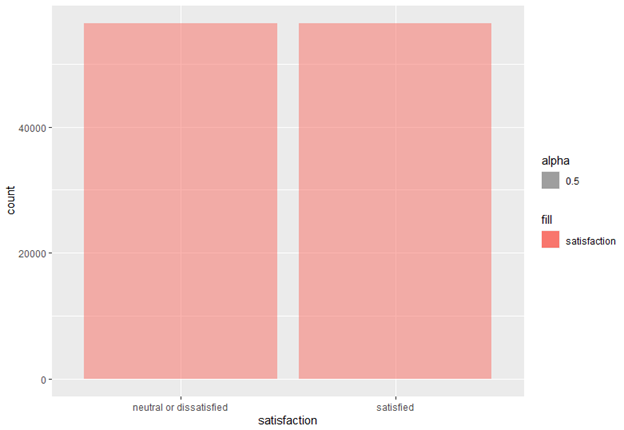The first part of the EDA will include plotting the satisfaction variable to understand the balance of the dataset between the two levels of satisfaction. To further understand the relationships between the variables at a surface level a correlation matrix will also be plotted as this will assist to understand the relationships between different variables. The final part of the EDA will include plotting of missing variables through the dataexplorer library. After the EDA has been conducted the pre-processing of data begins. To pre-process the data, firstly mutate_all function from dplyr will be used to mutate any blank values to na values to be imputed in the next step. After all the blank values have been converted to na values the mice library will impute the missing values. Mice utilizes a various algorithms such as classification and regression trees (CART) algorithms to predict the missing values based on the other factors (Hong & Lynn, 2020). After all the missing values have been imputed, normalization of the data will take place. A min-max normalization method is used for this case as it converts all numeric variables to a scale between 0 and 1. This is done through the formula (value-minimum value) / (maximum value – minimum value) (Loukas, 2020). After min-max scaling has been completed, the last step of preprocessing will involve balancing the dataset through under sampling. As the dataset is large, under sampling will remove the observations with the class with more observations so that it is equal to the class with fewer observations.

Machine Learning Techniques

To keeping consistency among all the algorithms being evaluated, all the algorithms will be executed through the caret library with the same control (k-fold cross validation) function. Caret library is machine learning library for R programming language that can execute various machine learning algorithms with the help of external machine learning libraries (Prabhakaran, 2018). Caret also has an inbuilt trainControl function that helps to set parameters for cross validation and tuneLength parameter that helps to set tuning parameters. The trainControl function of all the algorithms will be set to 10 fold repeated cross validation with 5 repeats. The search parameter within trainControl which searches for tuning parameters within the algorithm will be set to random as this will check a more diverse range of values to tune the algorithm.

Naïve Bayes

The Naïve Bayes algorithm is the most basic model being implemented in this study and the algorithm for the Naïve Bayes implementation will be loaded from the klaR library as this library supports the implementation of the algorithm from the caret library. The hyperparameters that need to be tuned in Naïve Bayes include the Laplacian correction factor, Usekernel parameter that chooses between gaussian and nonparametric distribution and adjust or the bandwidth adjustment parameter.

Decision Trees

The library to be used for the decision tree modelling is the ‘rPart” library. The tuning length for the model is set for 10 with the only tuning parameter for the model being the complexity parameter cp which will be randomly explored during the model tuning phase. Artificial Neural Network The library for the neural network modelling will be the nnet library. The tuning parameters for the ANN model will be the hidden layers parameter and the weight decay parameter. The hidden layers parameter tunes the model on the number of layers in the hidden layer of the neural net.

Evaluation Methods

To evaluate the models, various aspects of the model will be explored. The most basic evaluation method do be used is the accuracy metric which simply outputs the percentage of the correct predictions from the total number of predictions. However, the accuracy measure may prove to be a bit misleading as it can output more true positives compared to true negatives if it contributes to the accuracy metric to become larger. Hence along with the accuracy, the sensitivity and specificity metric will also be used to compare the percentage of true positives and true negatives. As it is difficult to compare the two specificity and sensitivity metric objectively, the F-measure will be used to compare it. However, as the dataset has already been balanced for this particular dataset, it is unlikely for the model to be more biased towards one class over the other (Brownlee 2020). The final evaluation metric to be used for this study is the Receiver Operating Characteristics (ROC) Curve and the Area Under the receiver operating characteristics Curve (AUC). The ROC is a probability curve that displays the false positive rate against the false negative rate at various probability thresholds (Narkhede, 2018). The AUC, utilising the ROC outputs the measure of separability of the classifier. Hence, the higher the AUC the better the classifier, which will be a metric used to measure the best model in this study.

Data Preparation

Initial EDA

library(dplyr)
library(DataExplorer)
library(mice)
library(VIM)
library(missForest)

The Data-preparation begins by importing data cleaning libraries such as dplyr, mice, VIM and missForest as well as data exploration library DataExplorer to understand the data better.

df <- read.csv ('Full_DS.csv', header=T) 

View(df)
str(df)
summary(df)

After importing the libraries, the working directory is set to the folder where the dataset is located. This allows for easier reading of the dataset. The dataset is a csv file hence, read.csv command is used to load the dataset and is assigned to the variable df.

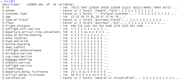
To check if the dataset was loaded correctly, the data set is viewed through the view command. Followed by that, the structure and summary of the data is viewed to check the format and structure of the data including important summaries such as frequency, averages and standard errors of the variables.

The structure of the data confirms the previous description of the dataset highlighted in the methodology section of this paper including number of observations and variables. However, as the dataset imports non-numeric variables as character values, this needs to be converted into factor variables to better understand the structure of the data including the number of levels in these variables to allow for dummification in variables where it is needed.

The summary of dataset reveals important details of the dataset especially for the numeric variables including the minimum and maximum values, mean, median as well as the quadrants. For character variables the summary function reveals the number of observations as well as the class of the variables.

df$Gender = factor(df$Gender)
df$Customer.Type = factor(df$Customer.Type)
df$Type.of.Travel = factor(df$Type.of.Travel)
df$Class = factor(df$Class)
df$satisfaction = factor(df$satisfaction)

str(df)

levels(df$Gender)
levels(df$Customer.Type)
levels(df$Type.of.Travel)
levels(df$Class)
levels(df$satisfaction)

All the character variables in the dataset are converted to factor variables using the factor command. As these values are stored back in the dataset, the structure of dataset is checked again through the str function. To further analyze the factors to check for consistency of the data, the levels of the factor variables are also checked to assess if missing values are classified as a level.

Figure 1:

After factorization is completed, all the character variables can be observed as factors with either 2 or 3 levels in each variable.

Pre-Processing

budf <-df

df <- mutate_all(df, na_if, "")

plot_missing(df)

Before moving further with imputing missing data, a backup of the dataset is created to ensure that if dataset needs to be reverted to its original form, the backup will be available. After backing up, the dataset is mutated to convert blank values to na values to ensure that no values are missed.

imputed_df <- mice(df, m=3)
Final_imputed_df <- complete (imputed_df)

#Check the imputed DF for missing values
plot_missing(Final_imputed_df)

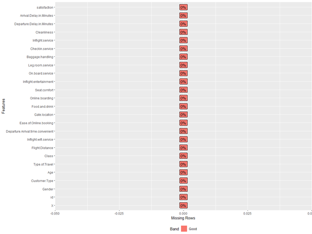
To impute the missing values for this project the MICE library is used with the m value (Number of multiple imputations) set for 3. After the mice imputation is initialized the complete function is used to fill in the missing data and return the completed data. After imputation is completed the missing value plot is once again plotted to check the new imputed data for missing values

Figure 2

There are no missing data after data has been imputed.

library(fastDummies)

dummied <- dummy_cols(ddf, remove_first_dummy = TRUE)

data <- dummied[c(-2,-3,-5,-6,-24)]
str(data)

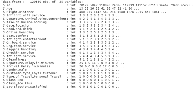
To dummy encode the data, fastDummies library is loaded and a new data frame named dummied is created to store the dummy encoded data for all categorical variables. The remove_first_dummy parameter is set to True, which removes creates columns for 1 – number of levels. After encoding, the factor variables are removed leaving the data frame full of integer values and is saved in a dataframe named data. To ensure that only integer values are present in the dataset the structure is checked.

Figure 3

After encoding is complete, we are left with a clean dataset with only integer variables.

#define Min-Max normalization function
min_max_norm <- function(x) {
  (x - min(x)) / (max(x) - min(x))
}

#apply Min-Max normalization to all the columns
norm.data <- as.data.frame(lapply(data, min_max_norm))

One of the common problem faced during Machine Learning Modelling is having data that has not been normalized. This can lead to variables with large numeric values to be given unequal weight when compared to variables with smaller numeric values. After the Min-Max normalization is applied the data is stored in norm.data completing the pre-processing of data for modelling. This data frame will be renamed to df for simplicity of the modelling process.

Balancing

satisfied <- which(norm.data$satisfaction_satisfied == 1)
dissatisfied <- which(norm.data$satisfaction == 0)

length(satisfied)
length(dissatisfied)

undersample <- sample(dissatisfied,length(satisfied))

undersampled <- norm.data[c(undersample,satisfied),]

library(ggplot2)

ggplot(undersampled) + 
  geom_bar(aes(x=satisfaction_satisfied,  alpha=0.5, fill='satisfaction'))

To do so firstly, the indices of the passengers in both classes are extracted through the which command and their length is checked to ensure that there are fewer satisfied passengers compared to dissatisfied passengers. After this, a random sample of the indices from the neutral or dissatisfied class of the same length as the satisfied class is extracted. This sample along with the satisfied class is compiled into a dataframe named undersampled is created and once again the data distribution for the classes are created to check for the balance.

The new plot reveals that both classes are of equal length now. However, due to the large size of the dataset, training times for this model become unrealistically high for a project of this scale. For this reason, a sample of the full dataset will be extracted for all the models to be used uniformly for both testing and training of the model. The same test data will be used to evaluate and compare all the models. Both the test and training datasets are then exported to allow for consistency when being used for modelling.

set.seed(16)

split = sample.split(df, SplitRatio = 0.1)
ndf = subset(df, split = TRUE)

split = sample.split(ndf, SplitRatio = 0.5)
ndf = subset(df, split = TRUE)

split = sample.split(ndf, SplitRatio = 0.7)
training_set = subset(ndf, split = TRUE)
test_set = subset(ndf, split = FALSE)

Experimentation and modelling of ML models

Naive Bayes

Naïve Bayes will be the first model that will be implemented for the prediction as it is the most simple of the three algorithms. The algorithm will be modelled through KlaR library and implemented in the caret train model using 10 fold cross validation on the training set.

install.packages('klaR')
library("klaR")

control <- trainControl(method="repeatedcv", number=10, repeats=5, search="random")

The most important steps that need to be taken before modeling of a Machine Learning algorithm is to set the validation techniques and parameters. For the decision tree model the trainControl from Caret library is used with repeated cross validation (repeatedcv). The number 10 indicates that the dataset was split across 10 divisions and repeated 5 times. The search parameter is set for random to ensure that the cp value to be tuned is not selected in a systematic manner, but randomly increasing the chances of finding the best value for the algorithm.

Naive.Flights = train(satisfaction_satisfied ~ ., 
                      data=training_set, 
                      method="nb", 
                      trControl = control,
                      tuneLength=10)

After setting the initial crossvalidation parameters the modelling of the naïve bayes algorithm takes place. The model is saved as Naïve.Flights.

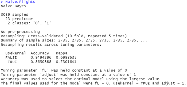
After the model is finished training the model is displayed to reveal details of the tuning and final model. A total of 3039 samples were available for training with 23 predictors and 2 classes. As repeated Cross validation took place, it evaluated the accuracy for just the usekernel (distribution type) parameter. However, there are other hyperparameters that were not tuned, namely the fL (Laplace Correction) and adjust (bandwidth adjustment) parameter. Hence, a second model will be created to tune the two remaining parameters.

nbgrid <-  expand.grid(fL = c(0,0.5,1), 
                       usekernel = c(TRUE,FALSE),
                       adjust = c(0.5,1,2,2.5,3))

Naive.Flights = train(satisfaction_satisfied ~ ., 
                      data=training_set, 
                      method="nb", 
                      trControl = control,
                      tuneGrid=nbgrid)

Naive.Flights

plot(Naive.Flights)

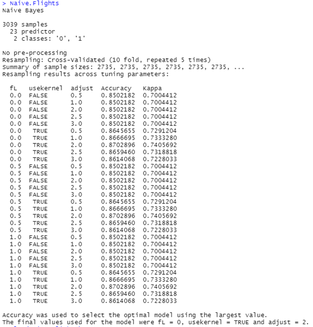
Using the same repeated cross validation as the control, a tune grid is created and a list of parameters are entered to tune the algorithm based on these parameters.

When the model is implemented, the model is tuned based on all possible combination of parameters based on the list of value entered in the tune grid. However, after analysing the accuracy of all possible combination, the model has concluded that the best model is the initial model with a change in adjust parameter to 2.

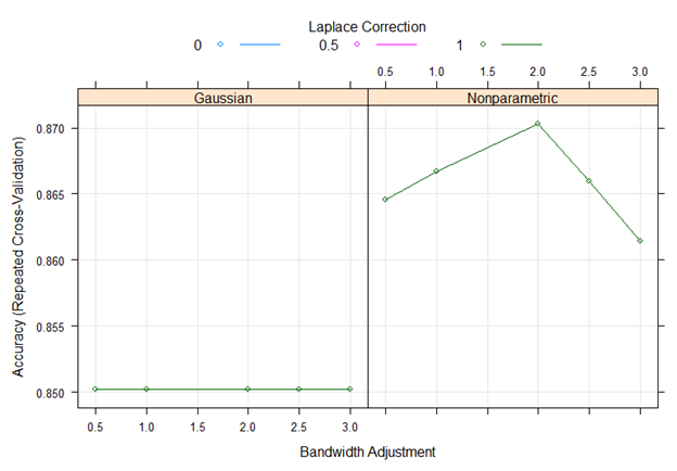
When the model is plotted, it displays the outcome of the tuning based on whether the usekernel was Gaussian on Nonparametric. It shows that once again the best performing model was Nonparametric model. It also shows that the Laplace Correction has no influence on the accuracy of the model with the bandwitdth adjustment having a significant influence on the model in nonparametric model as it increases the accuracy as the value is increased from 0.5 to 2. However, the model then experience a decrease in the accuracy after 2.0.

Decision Trees

The second model that will be evaluated using the pre-processed data will be the decision tree dataset.

library(caTools)
suppressMessages(library(rattle))
library(caret)

df <- training_set

To implement the Decision Trees Model, the caret library along with rattle library loaded in suppressmessages command to visualize the decision tree efficiently. Followed by this the balanced dataframe will be once again renamed to df before modelling starts.

control <- trainControl(method="repeatedcv", number=10, repeats=5, search="random")

flight.tree = train(satisfaction_satisfied ~ ., 
                    data=df, 
                    method="rpart", 
                    trControl = control,
                    tuneLength=10)

As already described in the first Naïve Bayes model, the same control parameters are used for training this model as well to ensure that all models are evaluated at the same level. To model the decision tree, the train function from caret library is called and the dependent variable from the data frame that was normalized for modelling (df) is selected. The data is specified as df. As the model selected is a decision tree Recursive Partitioning and Regression Trees (rpart) is selected as the method of the model. The trControl parameter is set for the validation and tuning parameters that was set in the previous step. Lastly the tune length is set at 10 ensuring that 10 different CP values will be selected at random to select the best value.

flight.tree

confusionMatrix(flight.tree)

After the training is complete, the model evaluation is conducted by displaying a summary of the tuning and validation on the model as well as displaying the confusion matrix. The confusion matrix is displayed using the Caret library.

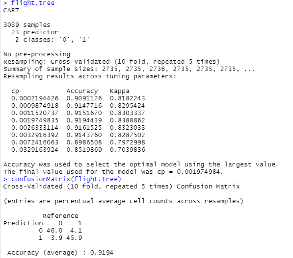
When the model is called it displays the summary of the evaluation including the number of samples that were used in modelling (112856), using 23 predictors to predict 2 classes. Furthermore, it also displays the sample size of the splits used when modelling using kfold validation with each kfold validation repeated 5 times and displaying the average for each of the 10 CP Values. The best CP Value is chosen based on the accuracy of the model. Although in table form with various numbers, it is difficult to interpret the CP Value and accuracy trend this will be visualized in the next step.

When looking at the confusion matrix, as this was displayed using the model, it shows the percentages which makes it easier to interpret the matrix. As the dataset was perfectly balanced (50/50 for each class), doubling the True Positive and True Negative values provide the sensitivity and specificity values respectively. The model has a 91.94% accuracy with 0.92 sensitivity value and 0.918 specificity value.

fancyRpartPlot(flight.tree$finalModel)

plot(flight.tree)

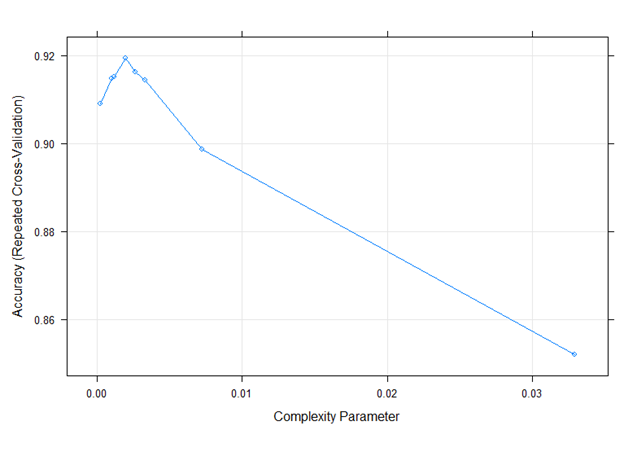
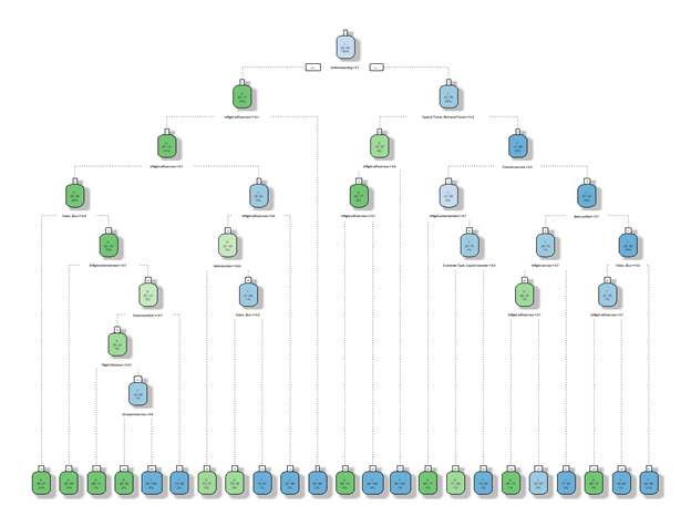
To visualize the model, firstly the model is plotted to analyse the trends associated different CP values and accuracy. Furthermore fancyRpartPlot from rattle is used to visualize the final model from the flight.tree model.

The model plot shows how the algorithm derived the complexity parameter 0.00197 as it shows that, it was the value with the highest accuracy with the accuracy dropping on either side of that value.

Visualization of the Decision Tree shows the different branches the algorithm takes to reach each of its conclusion.

Artificial Neural Network

The same dataset used for the previous two models was also used to model the Artificial Neural Network (ANN) model in the same Caret library using the nnet library as the method.

library(caTools)
library (nnet)

control <- trainControl(method="repeatedcv", number=10, repeats=5, search="random")

ann <- train(satisfaction_satisfied ~., 
             data = df, 
             method = "nnet", 
             trControl = control)

ann
plot(ann)

After loading the dataset and libraries the indices from the dataset is removed and the dependent variable is converted to a 2 level factor to allow for classification modeling.

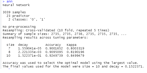
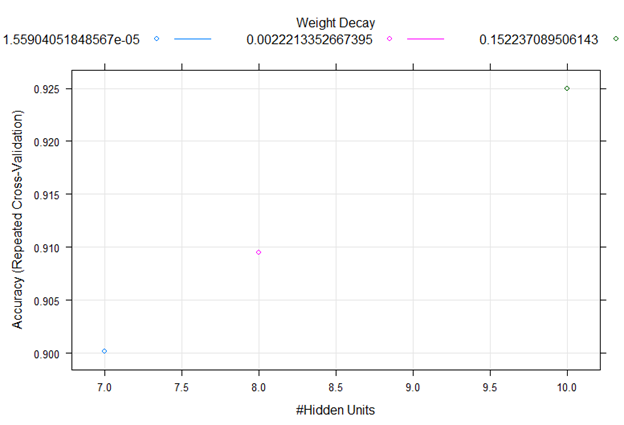
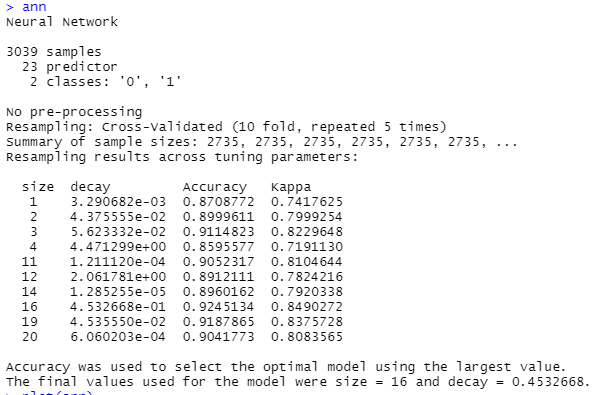
To model the ANN, the same control measures as previous models were used to keep consistency. After training the model it is saved in variable ann which is called after training is complete to assess the performance of the model. The model is also plotted to visualize the result of the model

As seen, in the summary, using accuracy as the metric to identify the optimal model, three different values were randomly chosen for size and decay values with varying degrees of accuracy for each model. Hence another tuning iteration will be implemented with tuning length set as 10 to ensure that more variables are tried and tested to identify the best parameters.

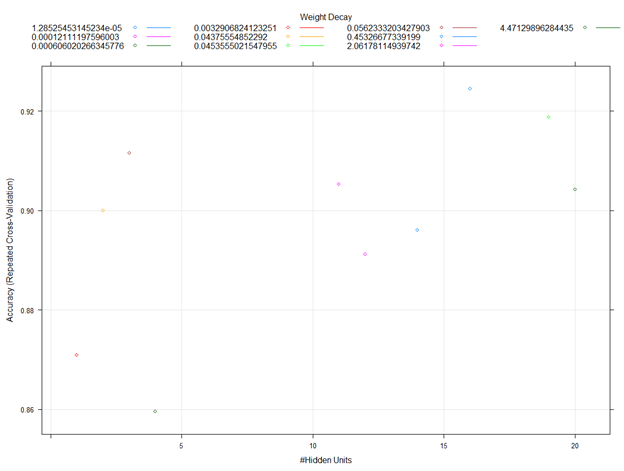
The visualization of the model shows that there is a direct correlation between accuracy and the number of hidden units. However, it must also be noted that this also has varying weight decay values. Hence more tuning is needed to identify the best model.

control <- trainControl(method="repeatedcv", number=10, repeats=5, search="random")

ann <- train(satisfaction_satisfied ~., 
             data = df, 
             method = "nnet", 
             trControl = control,
             tuneLength = 10)

For the final tuning of the ANN model, the same cross validation parameters are used, however, tuneLength parameter is set to 10 which randomly chooses 10 different values for size and decay variables and combines them to find the accuracies to identify the optimal model.

Using this technique the model was evaluated to find the best parameters. The best performing model from the different parameters was the model with 16 hidden layers and decay value of 0.45. This model was further plotted to check for any further trends.

The plot shows that the model is highly volatile and varies with both hidden units and weight of decay. The plot confirms the highest accuracy was obtained with 16 hidden units and 0.45 set as weight decay.

install.packages('NeuralNetTools')  
library(NeuralNetTools)  
plotnet(ann, alpha = 0.6)  

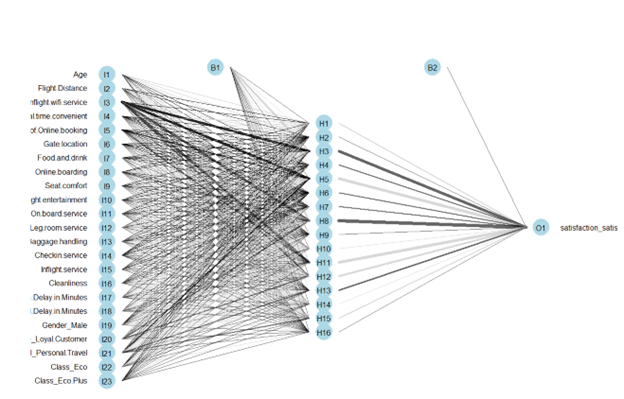
To further display the structure of the Neural Net, it is visualized using the NeuralNetTools showing the weights from each variable to the hidden layers and from hidden layers to the final classification.

The final step was saving the model to be loaded again to do the final evaluation with the test dataset that was created during the data-preprocessing step.

Evaluation

The final stage of Machine Learning implementation is to compare different models and identify the best performing model. For the purpose of this study, accuracy, f_measure, ROC and AUC were used to compare and evaluate the different models.

library(pROC)
library(yardstick)
library(caret)

df <- test_set

As done for the modelling, first the libraries and dataset are loaded to the program. The libraries to be used for evaluating the models are pROC for displaying the ROC curve and calculate the AUC for each model. Furthermore, yardstick library will be used to obtain the F_Measure and Caret Library will be used to get predictions from the models.

Furthermore, as we will be using data that the model was not trained on before, and to maintain consistency and fair evaluation, same test data will be used for all the models.

naivemodel <- readRDS("naivemodel.rds")
dtmodel <- readRDS("dtmodel.rds")
annmodel <- readRDS("annmodel.rds")


##Prediction Naive Bayes
nmprob = predict(naivemodel,newdata = df[,-24],type='prob')
nmclass = predict(naivemodel,newdata = df[,-24],type='raw')

##Prediction Decision Trees
dtprob = predict(dtmodel,newdata = df[,-24],type='prob')
dtclass = predict(dtmodel,newdata = df[,-24],type='raw')

##Prediction Decision Trees
annprob = predict(annmodel,newdata = df[,-24],type='prob')
annclass = predict(annmodel,newdata = df[,-24],type='raw')

As all models were saved after being modeled for evaluation, the saved models were loaded to the program once again using readRDS function and saved into variables indicating the model name. After the models are loaded, each model is used to obtain predictions in both probability and class format. By default all classifications have a threshold of 0.5 for probability.

##Caret Confusion Matrix Evaluation NB
confusionMatrix(df$satisfaction_satisfied,nmclass)

##Caret Confusion Matrix Evaluation DT
confusionMatrix(df$satisfaction_satisfied,dtclass)

##Caret Confusion Matrix Evaluation ANN
confusionMatrix(df$satisfaction_satisfied,annclass)

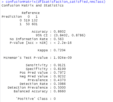
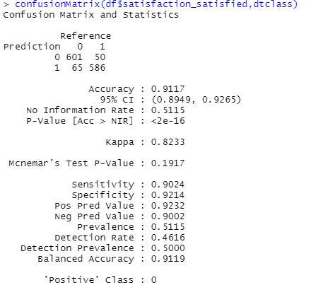
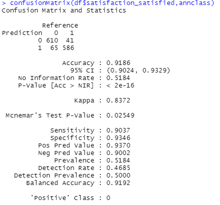
After all models obtain their predictions, a confusion matrix is created using the caret confusionMatrix tool that displays the analysis of the model performance.

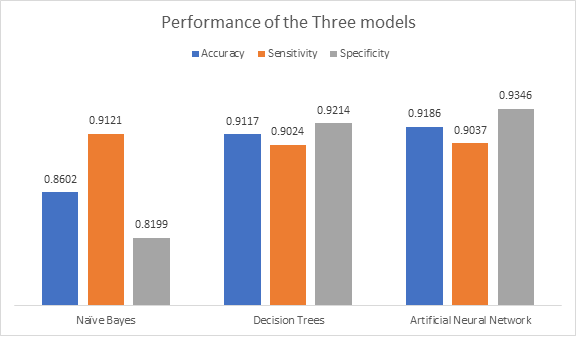
The first model, Naïve Bayes model performance shows an accuracy score of 0.86 with a sensitivity score of 0.91 and specificity score of 0.8199.

The Decision Tree model has performed better than the Naïve Bayes Model with an accuracy of 0.911 and a more balanced sensitivity to specificity ration of 0.90 and 0.92 respectively. Hence overall this model can be said to be a better performing model compared to the Naïve Bayes Model.

The final model, the Artificial Neural Network ANN model has also performed at a similar level to the Decision Tree model. However, the ANN model has a slightly higher accuracy than the Decision Tree model with 0.919 accuracy. The sensitivity and specificity for the ANN model is also in the 90s. to further evaluate the accuracy, the F score will be measured for each model.

As seen in the chart, it can be observed that the Naïve Bayes model has a more unbalanced prediction as it has a greater sensitivity compared to specificity. Both Decision Tree model and ANN model perform at a similar level in terms of accuracy, sensitivity and specificity.

##Yardstick F1 score (NBM)
nbeval = data.frame(df$satisfaction_satisfied)
nbeval$cl = nmclass
nbeval$pr = nmprob[,1]


f_meas(data = nbeval, estimate = nbeval$cl, truth = nbeval$df.satisfaction_satisfied)

##Yardstick F1 score (DTM)
dteval = data.frame(df$satisfaction_satisfied)
dteval$cl = dtclass
dteval$pr = dtprob[,1]


f_meas(data = dteval, estimate = dteval$cl, truth = dteval$df.satisfaction_satisfied)

##Yardstick F1 score (ANNM)
anneval = data.frame(df$satisfaction_satisfied)
anneval$cl = annclass
anneval$pr = annprob[,1]


f_meas(data = anneval, estimate = anneval$cl, truth = anneval$df.satisfaction_satisfied)

To evaluate the f measure from yardstick library first the predictions are inserted into a dataframe for easier processing. The F scores for each model is listed below.

As observed by the tables of F measure, Artificial Neural Network has the best F_Measure when compared to all other models.

plot1<- roc(df$satisfaction_satisfied, nbeval$pr, plot=TRUE, legacy.axes=TRUE,main="Naive Bayes ROC", percent=TRUE, 
            xlab = 'False Positive Percentage', ylab = 'True positive percentage', print.auc = TRUE,col = 'red')

plot2<-roc(df$satisfaction_satisfied, dteval$pr, plot=TRUE, legacy.axes=TRUE, percent=TRUE,main="Decision Tree ROC", 
           xlab = 'False Positive Percentage', ylab = 'True positive percentage', print.auc = TRUE,col='blue')

plot3<-roc(df$satisfaction_satisfied, anneval$pr, plot=TRUE, legacy.axes=TRUE, percent=TRUE, main="ANN ROC", 
           xlab = 'False Positive Percentage', ylab = 'True positive percentage', print.auc = TRUE,col='green')

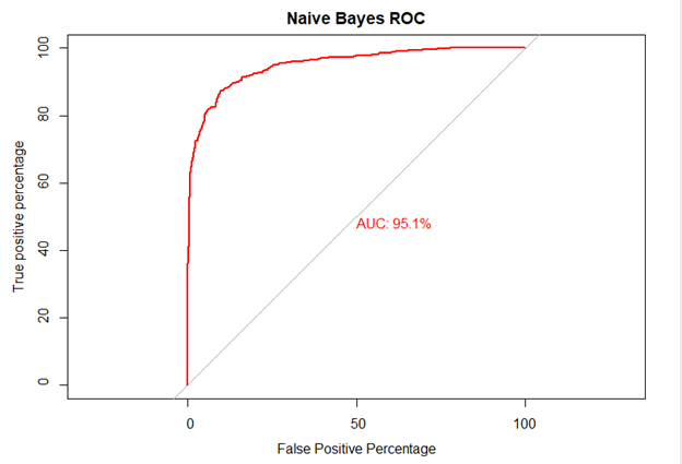
The last evaluation metric, ROC and AUC was plotted using pROC library and print.auc parameter was set to TRUE to allow the plot to display the value of auc for each plot.

The first plot of Naïve Bayes ROC shows a steady curve with an AUC of 95.1%

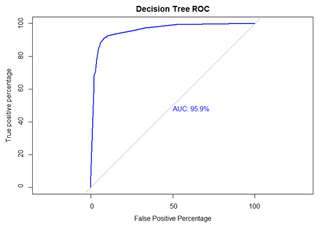
The Decision Tree has a sharper curve compared to the Naïve Bayes model with a better AUC of 95.9%.

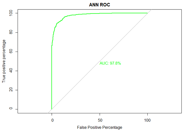
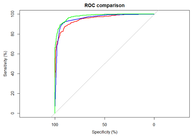
The final ANN Model has the best AUC with 97.8%. To compare the shape of the curves the three plots will be plotted together to evaluate it on a more graphical manner.

As seen in the AUC, once again it can be observed that the ANN, in green colour has the sharpest curve when compared to the other two models. Hence we can conclude that based on the accuracy, F measure, ROC and AUC, the Artificial Neural Network model has outperformed the Naïve Bayes model and the Decision Tree Model. The least significant of the three models is the simplest Naïve Bayes Model with Decision Tree model performing at a close level to the Artificial Neural Network Model.

importance <- varImp(annmodel, scale=FALSE)
importance
plot(importance)

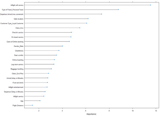
One of the objectives set for the study was to identify the most significant variables that contribute to customer satisfaction. Hence the most significant factors for the best performing model, the ANN was identified by using the varImp from caret library and plotted to visualize the features.

The plot reveals that the most important feature determining customer satisfaction is inflight wifi service followed by travelers travelling for personal purposes. The timing of the flight as well as gate location also plays an important factor in determining the customer satisfaction.

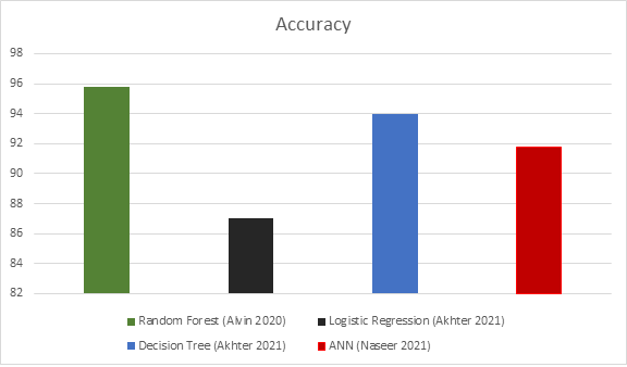
When comparing the implantation of the model against other implementations, we can observe that the previous implementations of the Random Forest and Decision Trees by other data scientists yielded higher accuracies where as logistic regression implemented by Akhter, (2021) underperformed compared to the current implementation. The main reason for the underperformance of the ANN model could be the use of a sample of the dataset rather than using the entire dataset for the training and testing of the model.

Conclusion

Due to the emerging challenges in the aviation industry due to the pandemic, airlines are having to compete in a depleted market for passengers. Increasing customer satisfaction was identified as a way to compete in this competitive market. To predict customer satisfaction and provide insight for airlines to improve their services, this study implemented a Naïve Bayes Classifier, a Decision Tree model, and an Artificial Neural Network model to predict customer satisfaction. After implementation and tuning of the model, the models were evaluated based on their accuracy, F measure and AUC. The three metric used for evaluation showed that the Artificial Neural Network model performed the best with the highest accuracy, F measure and AUC among the three models with the Decision Tree model performing closely. The Naïve Bayes model performed the worst among the three model. The ANN model also revealed the most significant features among the indicators with the inflight Wi-Fi being the most significant factor. When these models were compared with other models implemented using the same dataset, the model performed on average lower in terms of accuracy when compared to other models such as Decision Trees, and Random Forest models. However, the model did perform better than the Logistic Regression model. When analysing the reason for the model to perform weaker than other implementations, the most significant factor is that for this model the entire dataset was not used in training the models as for this study a sample of the dataset was used to optimise the training time. Hence, for further study, it is recommended that the entire dataset is used and analysed as this may improve the overall accuracy of the model. Lastly, in terms of business application of the findings, it is recommended that airlines focus their attention on the most significant predictors that have been identified through this model. Namely airlines should focus on the overall quality of Wi-Fi in airplanes as well as ensuring that the scheduling of flights are convenient for the customers instead of having flights at odd times of the day, especially flights with large number of passengers. It is also recommended that the airlines generally focus on improving the IT infrastructure of the airlines as passengers found ease of online boarding to be a significant factor in determining their overall satisfaction of the model as well.

References

An, M. & Noh, Y. (2009). Airline customer satisfaction and loyalty: impact of in-flight service quality, https://doi.org/10.1007/s11628-009-0068-4

Aitkenhead, M. J. (2008). A co-evolving decision tree classification method. Expert Systems with Applications, 34(1), 18–25. https://doi.org/10.1016/j.eswa.2006.08.008

Akhter, Z. (2021). Airline passenger satisfaction classification. [Kaggle Notedbook]. Retrieved from https://www.kaggle.com/chronicenigma/airline-passenger-satisfaction-classification

Alvin, T. P. (2020). Predicting Satisfaction of Airline Passengers with Classification. Retrieved from https://towardsdatascience.com/predicting-satisfaction-of-airline-passengers-with-classification-76f1516e1d16

Booma, P. M. & Wong, A. (2020). Optimising e-commerce customer satisfaction with machine learning. Journal of Physics Conference Series 1712. 10.1088/1742-6596/1712/1/012044

Bouwer, J., Saxon, S. & Wattkamp, N. (2021), Back to the future? Airlines sector poised for change post-COVID-19. https://www.mckinsey.com/industries/travel-logistics-and-infrastructure/our-insights/back-to-the-future-airline-sector-poised-for-change-post-covid-19

Brownlee. J. (2020). How to Calculate Precision, Recall, and F-Measure for Imbalanced Classification. Retrieved from https://machinelearningmastery.com/precision-recall-and-f-measure-for-imbalanced-classification/

Cho, K.-H., & Bae, H.-S. (2017). Convergence study of the in-flight meal quality on customer satisfaction, brand image and brand loyalty in airlines. Journal of the Korea Convergence Society , 8 (12), 317–327. https://doi.org/10.15207/JKCS.2017.8.12.317

Clemes, M. D., Gan, C., Kao, T. & Choong, M. (2008). An empirical analysis of customer satisfaction in international air travel. Innovative Marketing 4(2).

Curtis, T., Rhoades, D. L. & Waguespack, B. P. (2012). Satisfaction with Airline Service Quality: Familiarity Breeds Contempt. International Journal of Aviation Management, 1(4). https://doi.org/10.1504/ IJAM.2012.050472

Hong, S. & Lynn, H.S. (2020). Accuracy of random-forest-based imputation of missing data in the presence of non-normality, non-linearity, and interaction. BMC Medical Research Methodology 20(199). https://doi.org/10.1186/s12874-020-01080-1

John, D. (2016). Passenger Satisfaction (2.0) [Kaggle CSV dataset]. Retrieved from https://www.kaggle.com/johndddddd/customer-satisfaction/version/2

Kumar, S.& Zymbler, M. (2019). A machine learning approach to analyze customer satisfaction from airline tweets. Journal of Big Data 6(62). https://doi.org/10.1186/s40537-019-0224-1

Kwon, S. J. (Ed.). (2011). Artificial neural networks (Ser. Mathematics research developments). Nova Science. Retrieved December 11, 2021.

Loukas, S. (2020). Everything you need to know about Min-Max normalization: A Python tutorial. Retrieved from https://towardsdatascience.com/everything-you-need-to-know-about-min-max-normalization-in-python-b79592732b79

Mahmud, A., Jusoff, K. & Hadijah, S. (2013). The Effect of Service Quality and Price on Satisfaction and Loyalty of Customer of Commercial Flight Service Industry. World Applied Sciences Journal, 23(3), 354-359. 10.5829/idosi.wasj.2013.23.03.13052

Narkhede, S. (2018). Understanding AUC - ROC Curve. Retrieved from https://towardsdatascience.com/understanding-auc-roc-curve-68b2303cc9c5

Prabhakaran, S. (2018). Caret Package – A Practical Guide to Machine Learning in R. Retrieved from https://www.machinelearningplus.com/machine-learning/caret-package/

Ruan, D. (2006). Applied artificial intelligence : proceedings of the 7th international flins conference, genova, italy, 29-31 august 2006. World Scientific. Retrieved December 11, 2021.

Vazhavelil, T. (2020). How can the airline industry prepare for revival post COVID-19. https://www.wipro.com/blogs/thomas-vazhavelil/how-can-the-airline-industry-prepare-for-revival-post-covid-19/

Github repo

• Date: December 2021
• Assignment: Applied Machine Learning (Masters in Data Science and Business Analytics)
• Category: Machine Learning